Introduction

OpenFOAM is a powerful, open-source software tool used for computational fluid dynamics (CFD) simulations. It allows engineers and scientists to model and analyze the flow of fluids, such as gases and liquids, through intricate geometries and physical phenomena. For example, such physical phenomena could be turbulence, heat transfer, and chemical reactions. OpenFOAM has a large and dedicated user base and is utilized in a variety of industries, including aerospace, automotive, chemical, energy, and marine engineering.

This post focuses on the following challenges that users of OpenFOAM may encounter:

1. Complexity: OpenFOAM is a highly flexible and powerful tool, but this can also make it difficult for new users to learn and navigate. The software has a large number of solvers and utilities, and it can be challenging to understand which solver is most suitable for a given problem.

2. Data management: OpenFOAM simulations generate a number of outputs that need to be stored, versioned, shared, and cleaned up when needed.

3. Interfacing with other software: OpenFOAM may need to be used in conjunction with other software, such as CAD or mesh generation tools, and there can be challenges in integrating these tools and transferring data between them.

4. Software version control: OpenFOAM and simulation software are constantly updating and very complex software packages.

All challenges above become more challenging for a small team of researchers who develop and run simulations. They may lack experience with DevOps and cloud Infrastructure management. Therefore, having a handy toolset is needed to help with pipelines and infrastructure setup.

With DVC you may manage versions of simulation outputs, pipelines, and control software versions used to execute the pipeline ensuring consistent results. These features allow users to ensure that the new version of the software produces the same results as previous versions, helping to maintain the reliability and accuracy of the simulations. CML and Iterative Studio together provide a key for cloud resources management, running new experiments via nice UI, showing parameters and results of the simulation.

We describe these and other features in the two following posts. In this post, we discuss how Iterative tools help with physical and computational simulations. To do this, we’ll go over a simple demo project built with OpenFOAM. The demo shows how to set up DVC for simulation experiments and data management.

These posts are a result of collaboration between the Iterative.ai and PlasmaSolve teams. PlasmaSolve was founded in 2016 by plasma physicists and software engineers to provide a platform for cutting-edge physics simulation services and research. The PlasmaSolve team strives to deliver top-notch solutions and well-designed physics simulations to speed up research and reduce development costs using various open-source and commercial simulation tools.

In this post, you will learn how to:

1. Configure and run OpenFOAM simulations with DVC

2. Store and share simulation data in the cloud using DVC

sonicFoam simulation pipeline

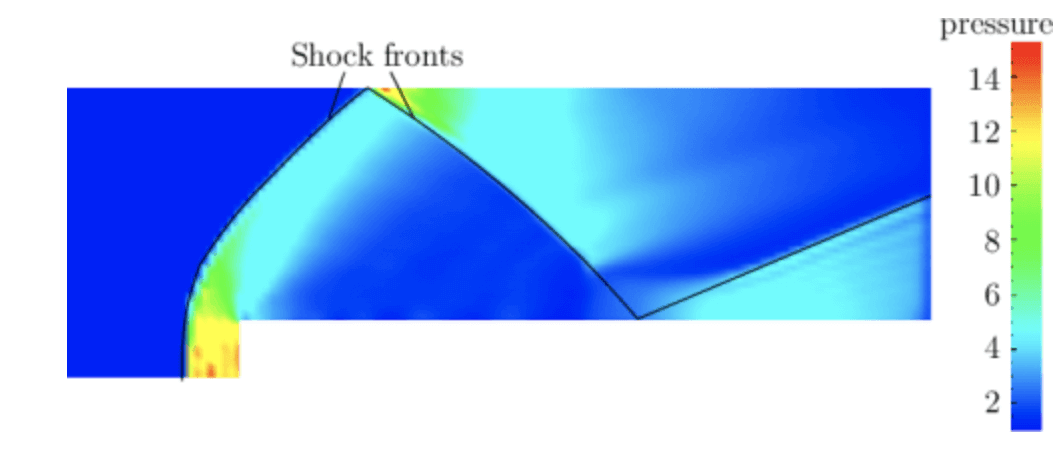
OpenFOAM simulations may include several computational steps, from mesh generation to a large number of solvers and post-processing simulation results. SonicFoam is a simulation tool based on the open-source CFD (Computational Fluid Dynamics) software OpenFOAM. It is used to simulate compressible, inviscid flows with high Mach numbers, such as supersonic flows.

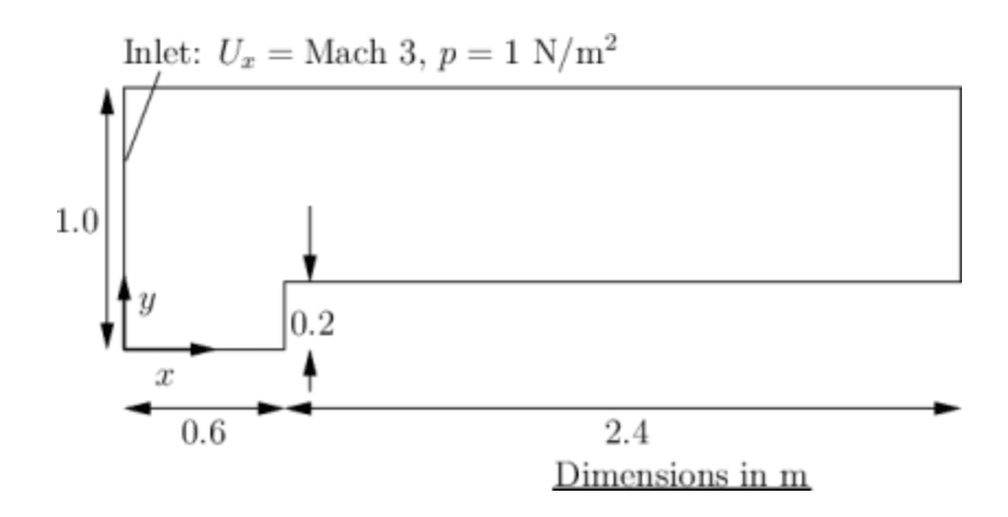
In this demo, we simulate a supersonic flow over a step located at the front of the flow. The scenario involves a Mach 3 flow entering a rectangular area with a step near the inlet, which creates shock waves. We use the same geometry to run two chained simulations: sonicFoam and scalarTransportFoam.

Shock fronts in the forward step problem (source)

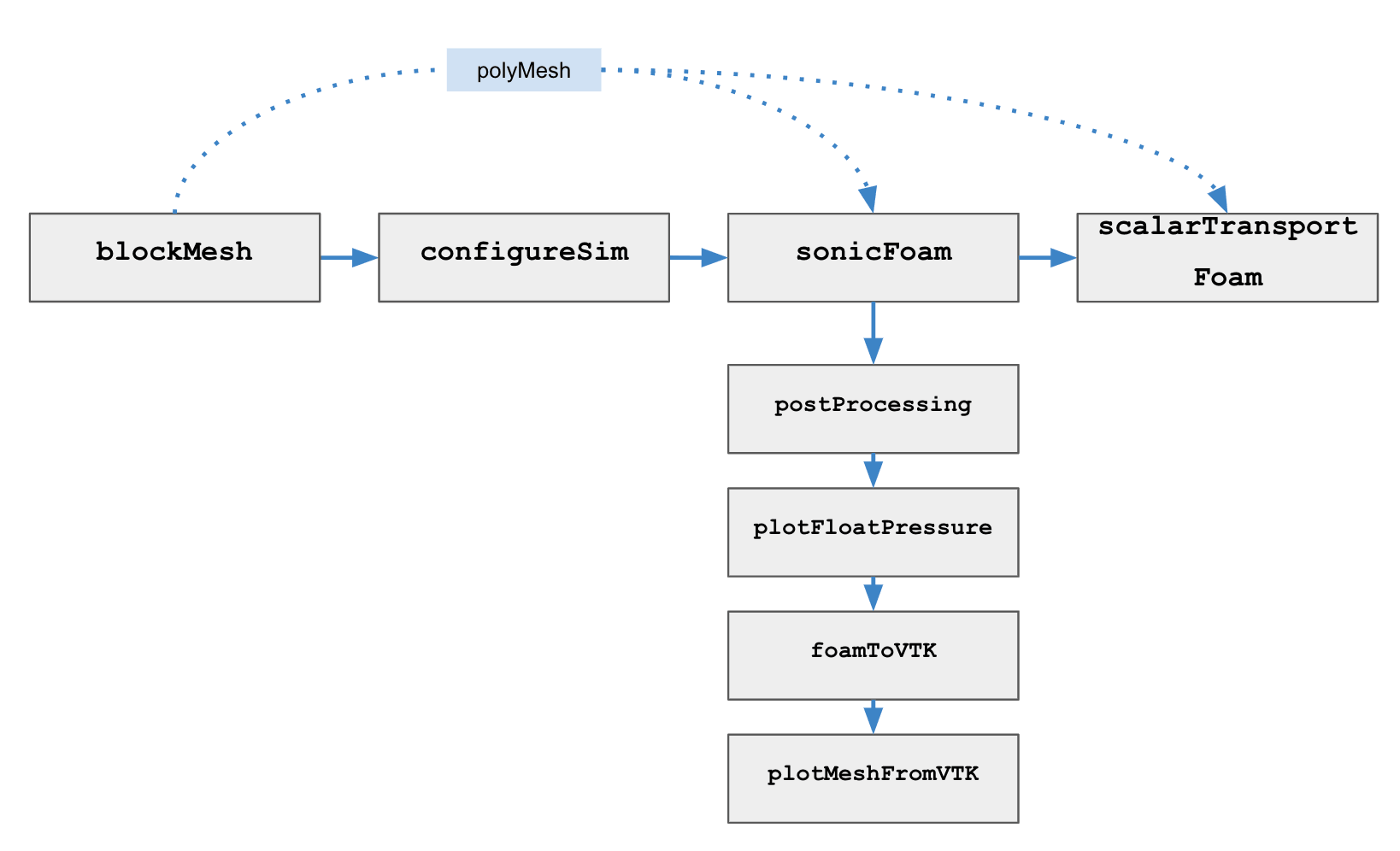
Our demo simulation pipeline contains a few steps:

1. Generate geometry with blockMesh;

2. Run sonicFoam simulation to get velocity (U) and temperature (T) fields;

3. Post-processing simulation results;

4. Run a subsequent scalarTransportFoam simulation that uses the velocity field computed before.

In reality, simulations sometimes need to be “chained”, i.e. outputs of one simulation go as an input to another simulation. When running a parametric study of such a simulation chain, intermediate simulations are often recomputed even if the parameter change does not influence them. We demonstrate how to use DVC to cache all the results and only trigger a computation if really necessary. Results of the sonicFoam solver go as inputs to the scalarTransportFoam solver.

As a basis for the demo, we use OpenFOAM Supersonic flow over a forward-facing step tutorial. The original code can be found here.

Setup the demo project

💡 For this part of the post, we follow the no-dvc branch in the demo repository.

The easiest way to follow the demo with OpenFOAM simulation is to run in Docker containers. Follow the setup section in the repository README to build a Docker image and set up Python virtual environment and install dependencies.

After the environment is set up we only need to run openfoam-cse-docker script which runs a new OpenFOAM job in a Docker container. For example, to run the OpenFOAM simulation in an interactive way, use the command:

$ ./openfoam-cse-docker

1. Generate geometry with blockMesh

To use sonicFoam, a user must first create a 3D geometry model of the flow domain using a tool such as CAD software. The user must then define the boundary conditions and physical properties of the flow, such as the temperature, pressure, and velocity at each boundary. The user can then run the simulation using the sonicFoam solver, which will solve the governing equations of compressible flow using the finite volume method.

$ ./openfoam-cse-docker -c 'cd sonicFoam && blockMesh'

Geometry of the forward step (source)

2. Run the first step simulation with sonicFoam solver

During the simulation, sonicFoam will calculate various flow quantities, such as the pressure, velocity, and temperature, at each point in the flow domain. The user can then visualize and analyze these results using post-processing tools, such as ParaView, to gain insight into the flow behavior.

$ ./openfoam-cse-docker -c 'cd sonicFoam && sonicFoam'

3. Post-processing simulation results

As an example of post-processing stages in the simulation demo, we have a few tasks:

• calculate the magnitude of the velocity

• calculate flowRatePatch

• generate VTK and visualize mesh

Calculate the magnitude of the velocity

postProcess is a command allows users to perform post-processing operations on simulation data. The -func option specifies that a user-defined function should be applied to the data. In this case calculates and writes the field of the magnitude of velocity into a file named mag(U) in each time directory generated during simulation:

$ ./openfoam-cse-docker -c 'cd sonicFoam && postProcess -func "mag(U)"'

The postProcess command can be used in conjunction with various options and functions to perform a wide range of post-processing tasks, such as calculating flow quantities, generating plots, and creating animations. It is an important tool for gaining insight into the results of CFD simulations.

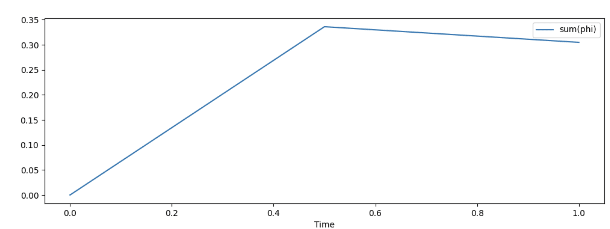
Calculate flowRatePatch

In order to produce a 1D dataset and its visualization we compute the flow rate over the “outlet” patch. For this purpose, we may apply the flowRatePatch(name=outlet) function to the simulation data. The flowRatePatch function calculates the flow rate through a patch, which is a specified boundary in the flow domain. The input name specifies the patch to use, in this case, outlet. The outlet patch represents the boundary at the outlet of the flow domain, so the flowRatePatch function will calculate the flow rate through the outlet.

$ ./openfoam-cse-docker -c 'cd sonicFoam && \
     postProcess -func "flowRatePatch(name=outlet)"'

This operation saves results into the sonicFoam/postProcessing/flowRatePatch(name=outlet)/0/surfaceFieldValue.dat file.

Generate VTK

foamToVTK is a utility converts simulation data stored in the OpenFOAM format to the VTK (Visualization ToolKit) format. VTK is a popular file format for storing and visualizing scientific data, and it is often used for post-processing and visualization of CFD simulations.

$ ./openfoam-cse-docker -c 'cd sonicFoam && foamToVTK'

This will convert the simulation data stored in the sonicFoam directory from the OpenFOAM format to the VTK format, allowing it to be visualized and analyzed using tools that support the VTK format. It creates sonicFoam/VTK/ directory with formatted simulation results.

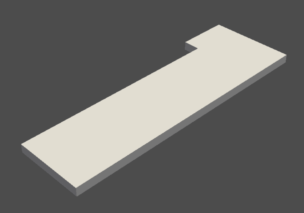
4. Visualize simulation results

To visualize the results of a simulation performed using the OpenFOAM toolkit's sonicFoam solver, you can use one of the post-processing tools included with the OpenFOAM toolkit, such as paraFoam or foamToVTK. These tools allow you to view and analyze the simulation results in a graphical interface.

In the demo example, a 3D geometry mesh and float pressure diagram are generated. There are examples of generated files below.

3D mesh visualization

Float pressure diagram

5. Run the second step simulation with scalarTransportFoam solver

The scalarTransportFoam is a solver in the open-source CFD software OpenFOAM that is used to solve a transport equation for a passive scalar using a specified stationary velocity field. It is typically used to calculate the convection diffusion of a scalar in a given velocity field.

Before running scalarTransportFoam solver, we need to update the stage configuration based on the sonicFoam outputs:

• Copy U config from the last simulation stage in sonicFoam

• Update T config with the boundaryField from the last simulation stage in sonicFoam

• Copy the polyMesh to use the same geometry

# Configure scalarTransportFoam
$ python3 src/config_scalarTransportFoam.py

# Run scalarTransportFoam simulation
$ ./openfoam-cse-docker -c 'cd scalarTransportFoam && scalarTransportFoam'

The simulation will calculate the transport of the passive scalar using the specified velocity field and other input parameters. The resulting simulation data can then be post-processed and analyzed to gain insight into the transport of the scalar in the flow.

Reduce simulation management complexity with DVC

💡 For this part of the post, we follow the main branch in the demo repository. Please follow the README to prepare your environment and install dependencies.

Up to this moment, we run different tasks for the simulation pipeline using separate commands. Let’s see how DVC tools can help with automating the simulation pipeline and handling simulation output data.

DVC pipelines is a feature of the DVC (Data Version Control) tool. A DVC pipeline is a series of commands that are executed in a specific order and can be used to run all steps that are needed- simulation itself, post-processing the results, and generating reports. DVC automatically captures and tracks the data and code associated with your OpenFOAM simulations to make them reproducible and shareable with your team.

Basic computational stage configuration

A DVC config file is written in YAML format and consists of a list of steps, each of which corresponds to a command that should be executed as part of the pipeline. The steps can depend on one another, meaning that the output from one step is used as input for another step. More details can be found on the DVC documentation website.

Let’s consider an example of the DVC pipeline configuration for blockMesh stage below.

blockMesh:
  cmd:
    - bash run.sh 'cd sonicFoam && blockMesh'
  deps:
    - sonicFoam/system/blockMeshDict
  outs:
    - sonicFoam/constant/polyMesh

The cmd field specifies the command to be executed, which in this case is a utility shell script run.sh that changes the file permissions and runs the blockMesh command directly or using openfoam-cse-docker script. The run.sh script “knows” how to run the simulations pipeline on your local environment (manually) or as a part of the GitLab CI pipeline on the Cloud environment (automatically). We will discuss CI configuration in later sections.

The deps field in this pipeline step specifies the input files that the blockMesh command depends on blockMeshDict file. These files contain information about the mesh and the simulation parameters, and are required by the blockMesh command to generate the mesh.

The outs field specifies the output files generated by the blockMesh command. In this case, the output is the polyMesh directory, which contains the generated mesh data. The mesh data is captured and versioned by DVC.

Configure simulation pipelines with params.yaml

DVC pipeline configuration file (params.yaml) file configures an OpenFOAM simulation. Here is an extract of the parameters used for sonicFoam stage configuration:

configureSim:
  sim_config_dir: configs
  controlDict:
    path: system/controlDict
    params:
      startTime: 0
      endTime: 3
      deltaT: 0.002
      writeInterval: 0.5
      purgeWrite: 0
      writePrecision: 5
      timePrecision: 6

The params field of the controlDict section specifies the values of the simulation control parameters. In this case, the startTime, endTime, deltaT, writeInterval, purgeWrite, writePrecision, and timePrecision parameters are set to specific values.

In the DVC simulation setup, the user is responsible for putting the values from the params.yaml file into the controlDict. Unlike other tools that handle this process automatically, this approach requires some manual effort on the user's end but provides greater flexibility as it eliminates the need for support for each and every tool or software used in the simulation. The demo showcases how this task is carried out through the src/configureSim.py script.

Adapt DVC behavior for the simulation use case

DVC pipeline configuration expects that all inputs and outputs of each stage are explicitly defined in the dvc.yaml file. This is a common pattern in Machine Learning and Data Management pipelines. DVC uses explicit deps and outs to build a computational DAG and “understand” whether it needs to re-run a stage if some of its dependencies change. This ensures the reproducibility of the pipeline.

However, OpenFOAM simulation pipelines are different. Depending on the simulation parameters (e.g. endTime and writeInterval in the controlDict parameters), a different number of files and folders can be generated. Therefore, it may impossible to specify all outputs in dvc.yaml in advance. But, because of these files are not specified in dvc.yaml, DVC can’t manage them properly. To solve this problem, we introduced two helper scripts that “help” DVC to find and handle generated files and folders for the simulation use case. Hopefully, supporting wildcard patterns in dvc.yaml configuration file will simplify such use cases!

Let’s introduce two additional helper scripts:

• dvc_outs_remove.py - removes the stage outputs from the previous simulation. This script checks if there are files previously added by dvc_outs_handler.py script and remove them from DVC with dvc remove command.
• dvc_outs_handler.py - finds all “untracked” and adds them to DVC control. By default, only files tracked by either Git or DVC are saved to the experiment. This script checks if there are files or directories generated by the stage and add them to DVC with dvc add command.

sonicFoam:
  cmd:
    # Remove previous sim results
    - python3 src/dvc_outs_remove.py --stage=sonicFoam ...

    # Run sim
    - bash run.sh 'cd sonicFoam && sonicFoam'

    # Add generated files to DVC and create outputs index files
    - python3 src/dvc_outs_handler.py --stage=sonicFoam ...
  params:
    - configureSim
  deps:
    - sonicFoam/constant/polyMesh/
    - ...
  outs:
    - ...

Link stages and multiple solvers

It is common for OpenFOAM simulations to involve complex pipelines with multiple steps and dependencies between the steps. This is because simulations often require the use of multiple solvers, each of which may have its own input and output files and dependencies on other solvers.

For example, a simulation may require the use of multiple solvers to simulate different physical phenomena, such as fluid flow, heat transfer, and chemical reactions. These solvers may need to be run in a specific order and may depend on the output of other solvers as input.

It’s possible to manage these dependencies with DVC! DVC allows you to specify the steps in the simulation pipeline and the dependencies between them in a configuration file.

The demo project example has two solvers: sonicFoam and scalarTransportFoam. Both solvers depend on the same geometry generated by the blockMesh stage. In the case we know exactly the path to the output (outs) of the sonicFoam solver, we may explicitly define it as a dependency (deps) of the scalarTransportFoam stage. In our case, we use a utility script (src/config_scalarTransportFoam.py) to get the results of the sonicFoam solver and prepare the initial state for the scalarTransportFoam solver.

scalarTransportFoam:
  cmd:
    - python3 src/config_scalarTransportFoam.py
    - ...
    - bash run.sh 'cd scalarTransportFoam && scalarTransportFoam'
    - ...
  deps:
    - sonicFoam/constant/polyMesh/
    - ...
  params:
    - plotMesh
    - scalarTransportFoam
  outs:
    - ...

Run a new simulation

After the DVC pipeline is set up, you may run a new simulation experiment with a command:

$ dvc exp run

To run a new simulation with updated parameters you may manually change the parameter value in the params.yaml file and run dvc exp run or, it’s possible to modify parameters on-the-fly. For example, let’s change the length of our simulation:

$ dvc exp run -S 'configureSim.controlDict.params.endTime=4'

It is also possible to queue and run multiple simulations in parallel.

In the next post, we will show how to visualize and compare simulation data with CML and Iterative Studio.

Versioning and sharing simulation data with DVC

Effective data management is essential for successful OpenFOAM simulations. Proper data management can help you organize and track the data and code associated with your simulations, and make it easier to reproduce simulation results.

There are several challenges that users of OpenFOAM may encounter in managing the data associated with their simulations:

1. Large data volumes: OpenFOAM simulations can generate large amounts of data, particularly for complex or high-resolution simulations. This can make it difficult to store, transfer, and analyze the data effectively.

2. Data version control: It is important for users to be able to track changes to the input files and simulation results over time and to be able to reproduce past simulations. This can be challenging without a version control system or other means of tracking changes.

3. Data transfer: Users may need to transfer large amounts of data between different systems or devices, such as between their personal computers and a high-performance computing cluster. This can be challenging due to the size of the data and the potential for data transfer bottlenecks.

4. Collaboration: Users may want to share simulation results with colleagues or collaborate on simulations. This can be done by sharing the simulation input files and results, as well as using tools such as online collaborative platforms or version control systems.

Luckily, DVC may help with all of them. Let’s review the core features of DVC that we used in the demo project. Data versioning is a core feature of DVC that helps to capture the versions of simulation data in Git commits, while storing them on-premises or in cloud storage. Moreover, using DVC pipelines, all outputs specified as outs, plots, or metrics in dvc.yaml configuration, are automatically added to DVC version control! Other files, generated by different stages, are added to DVC via dvc_outs_handler.py script. The next step is to set up DVC remote storage and upload these files there.

DVC help to store large volumes of data in the on-premise or cloud storage (e.g. SSH, S3, HDFS, etc.) The demo project uses AWS S3 as a remote storage. For more details on the remote storage configuration you may check Example: Customize an additional S3 remote.

You may add your own remote storage in AWS S3 bucket using the following command:

$ dvc remote modify s3remote url s3://<bucket>/<path>

After the remote storage is set up, you need a single additional command to transfer your results to the storage:

$ dvc exp push

With this DVC takes care of pushing and pulling to/from both Git and DVC remotes in the case of experiments. Therefore, the following collaboration with colleagues is simple. Your colleagues may access your last simulation results with a dvc exp pull command (after updating their repository with git pull):

$ dvc exp pull

Summary

This post details how Iterative tools help in physical and computational simulations. The demo shows how to set up DVC for simulation experiments and data management.

Overall, DVC can help OpenFOAM users to:

1. Reduce the complexity of simulation pipelines and automate tasks such as running simulations, post-processing results, and generating reports.

2. Manage and track the data and code associated with your OpenFOAM simulations, and make it easier to reproduce simulation results.

3. Manage simulation experiments with a YAML config files.

4. Store and share simulation data in the cloud using DVC and AWS S3.

5. Easily collaborate with your colleagues around simulation results, share and reuse data.

In the next post, we will discuss how to utilize cloud computing resources and visualize and compare simulation data with CML and Iterative Studio.